Tissot's indicatrix

View on a sphere: all are identical circles

Tissot's indicatrix (Tissot indicatrix, Tissot's ellipse, Tissot ellipse, ellipse of distortion) (plural: "Tissot's indicatrices") is a mathematical contrivance presented by French mathematician Nicolas Auguste Tissot in 1859 and 1871 in order to characterize local distortions due to map projection. It is the geometry that results from projecting a circle of infinitesimal radius from a curved geometric model, such as a globe, onto a map. Tissot proved that the resulting diagram is an ellipse whose axes indicate the two principal directions along which scale is maximal and minimal at that point on the map.

A single indicatrix describes the distortion at a single point. Because distortion varies across a map, generally Tissot's indicatrices are placed across a map to illustrate the spatial change in distortion. A common scheme places them at each intersection of displayed meridians and parallels. These schematics are important in the study of map projections, both to illustrate distortion and to provide the basis for the calculations that represent the magnitude of distortion precisely at each point.

There is a one-to-one correspondence between the Tissot indicatrix and the metric tensor of the map projection coordinate conversion.^[1]

Description

Tissot's theory was developed in the context of cartographic analysis. Generally the geometric model represents the Earth, and comes in the form of a sphere or ellipsoid.

Tissot's indicatrices illustrate linear, angular, and areal distortions of maps:

• A map distorts distances (linear distortion) wherever the quotient between the lengths of an infinitesimally short line as projected onto the projection surface, and as it originally is on the Earth model, deviates from unity. The quotient is called the scale factor. Unless the projection is conformal at the point being considered, the scale factor varies by direction around the point.
• A map distorts angles wherever the angles measured on the model of the Earth are not conserved in the projection. This is expressed by an ellipse of distortion which is not a circle.
• A map distorts areas wherever areas measured in the model of the Earth are not conserved in the projection. This is expressed by ellipses of distortion whose areas vary across the map.

In conformal maps, where each point preserves angles projected from the geometric model, the Tissot's indicatrices are all circles of size varying by location, possibly also with varying orientation (given the four circle quadrants split by meridians and parallels). In equal-area projections, where area proportions between objects are conserved, the Tissot's indicatrices all have the same area, though their shapes and orientations vary with location. In arbitrary projections, both area and shape vary across the map.

World maps comparing Tissot's indicatrices on some common projections
Equirectangular projection Mercator projection Gall–Peters projection Mollweide projection Winkel tripel projection Azimuthal equidistant projection Fuller projection Transverse Mercator projection Lambert cylindrical equal-area projection Sinusoidal projection Robinson projection Stereographic projection

Mathematics

Tissot's indicatrix

In the image to the right, ABCD is a circle with unit area defined in a spherical or ellipsoidal model of the Earth, and A′B′C′D′ is the Tissot's indicatrix that results from its projection on the plane. Segment OA is transformed in OA′, and segment OB is transformed in OB′. Linear scale is not conserved along these two directions, since OA′ is not equal to OA and OB′ is not equal to OB. Angle MOA, in the unit area circle, is transformed in angle M′OA′ in the distortion ellipse. Because M′OA′ ≠ MOA, we know that there is an angular distortion. The area of circle ABCD is, by definition, equal to 1. Because the area of ellipse A′B′ is less than 1, a distortion of area has occurred.

In dealing with a Tissot indicatrix, different notions of radius come into play. The first is the infinitesimal radius of the original circle. The resulting ellipse of distortion will also have infinitesimal radius, but by the mathematics of differentials, the ratios of these infinitesimal values are finite. So, for example, if the resulting ellipse of distortion is the same size of infinitesimal as on the sphere, then its radius is considered to be 1. Lastly, the size that the indicatrix gets drawn for human inspection on the map is arbitrary. When a network of indicatrices is drawn on a map, they are all scaled by the same arbitrary amount so that their sizes are proportionally correct.

Like M in the diagram, the axes from O along the parallel and along the meridian may undergo a change of length and a rotation when projecting. It is common in the literature to represent scale along the meridian as h and scale along the parallel as k, for a given point. Likewise, the angle between meridian and parallel might have changed from 90° to some other value. Indeed, unless the map is conformal, all angles except the one subtended by the semi-major axis and semi-minor axis of the ellipse might have changed. A particular angle will have changed the most, and value of that maximum change is known as the angular deformation, denoted as θ′. Generally which angle that is and how it is oriented do not figure prominently in distortion analysis. It is the value of the change that is significant. The values of h, k, and θ′ can be computed as follows.^[2]:24

$h = \frac{1}{R}\sqrt {{{\left( {\frac{{\partial x}}{{\partial \varphi }}} \right)}^2} + {{\left( {\frac{{\partial y}}{{\partial \varphi }}} \right)}^2}}$

$k = \frac{1}{{R\cos \varphi }}\sqrt {{{\left( {\frac{{\partial x}}{{\partial \lambda }}} \right)}^2} + {{\left( {\frac{{\partial y}}{{\partial \lambda }}} \right)}^2}}$

$\sin \theta ' = \frac{1}{{R^2 h k\cos \varphi }}\left( {\frac{{\partial y}}{{\partial \varphi }}\frac{{\partial x}}{{\partial \lambda }} - \frac{{\partial x}}{{\partial \varphi }}\frac{{\partial y}}{{\partial \lambda }}} \right)$

$a' = \sqrt {{h^2} + {k^2} + 2h k\sin \theta '}$

$b' = \sqrt {{h^2} + {k^2} - 2h k\sin \theta '}$

$a = \frac{{a' + b'}}{2}$

$b = \frac{{a' - b'}}{2}$

$s = h k \sin \theta '$

$\omega = 2 \arcsin\left({b' / a'}\right)$

where φ and λ are latitude and longitude, x and y are projected coordinates, and R is the radius of the globe.

As results, a and b represent the maximum and minimum scale factors at the point, s represents the amount of inflation or deflation in area (also given by a ∙ b), and ω represents the maximum angular distortion at the point.

For the Mercator projection, and any other conformal projection, h=k and θ′ = 90° so that each ellipse degenerates into a circle with the radius h=k being equal to the scale factor in any direction at that point.

For the sinusoidal projection, and any other equal-area projection, the semi-major axis of the ellipse is the reciprocal of the semi-minor axis so that every ellipse has the same area even though their eccentricities vary.

For arbitrary projections, neither the shape nor the area of the ellipses are related to each other in general.^[3]

Other distortion metrics

Many ways have been described for characterizing distortion in projections. Some, like Tissot's indicatrix, give visual indication of the distortion, such as the flexion and skewness (bending and lopsidedness) model.^[1]

The tiss-indicatrix approximates Tissot's indicatrix by using small circles (called 'tisses', meaning 'quick-and-dirty Tissot-indicatrix realization') instead of infinitesimal circles.^[4]

Averaged ratio between complementary profiles (AveRaComp) ${\tilde\rho _{CP}}\left( i \right)$ ^[5] gives a good estimation to Tissot's ω.

Firstly, planar grids (or cells) are constructed on projection plane(s), then the corners and center point of a given cell are transformed to sphere (or Reference ellipsoid). The corners on sphere are denoted as $P_j$, $j=1,\cdots,4$, and the center on sphere is denoted as $P_*$.

$\omega \approx {\tilde\rho _{CP}}\left( i \right) = \left[ {{\tilde\rho _{D3}}\left( i \right) + {\tilde\rho _\alpha }\left( i \right)} \right]/2$

where ${\tilde\rho _{D3}}\left( i \right)$ represents the ratio between diagonals, and ${\tilde\rho _{D3}}\left( i \right)$ represents the angle between diagonals.

${\tilde\rho _{D3}}\left( i \right) = \frac {{\max \left( {\left| {\overrightarrow {{P_1}{P_*}}} \right| + \left| {\overrightarrow {{P_*}{P_3}}} \right|, \left| {\overrightarrow {{P_2}{P_*}}} \right| + \left| {\overrightarrow {{P_*}{P_4}}} \right|} \right)}} {{\min \left( {\left| {\overrightarrow {{P_1}{P_*}}} \right| + \left| {\overrightarrow {{P_*}{P_3}}} \right|, \left| {\overrightarrow {{P_2}{P_*}}} \right| + \left| {\overrightarrow {{P_*}{P_4}}} \right|} \right)}}$

${\tilde\rho _\alpha }\left( i \right) = \cot \left( {\frac{1}{2}\arccos \left| { \frac{\overrightarrow {{P_1}{P_3}}}{\left| \overrightarrow {{P_1}{P_3}} \right|} \cdot \frac{\overrightarrow {{P_2}{P_4}}}{\left| \overrightarrow {{P_2}{P_4}} \right|} } \right|} \right)$

where $i$ is the index of a given cell on sphere (or Reference ellipsoid), $i=1,\cdots,N$, $N$ is the number of cells, and $\overrightarrow {{P_s}{P_t}}$ is a vector connecting points $P_s$ and $P_t$.

AveRaComp gives an simple form (via five points of cells, without differential calculus) to represent map distortions. It could also be used to evaluate non map projection based direct spherical subdivision (by using great circle arcs to subdivision a sphere).

Other visual methods project shapes that span a part of the map, rather than originally infinitesimal. In the first half of the 20th century, projecting a human head onto different projections was common to show how distortion varies across one projection as compared to another.^[6] Sometimes spherical triangles are used; sometimes other shapes. In dynamic media, shapes of familiar coastlines and boundaries can be dragged across an interactive map to show how the projection distorts sizes and shapes according to position on the map.^[7]

Another way to visualize local distortion is through grayscale or color gradations whose shade represents the value of the angular deformation or areal inflation. Sometimes both are shown simultaneously by blending two colors to create a bivariate map.^[8]

The problem of characterizing distortion globally across areas instead of at just a single point necessarily involves choosing priorities. Some schemes use distance distortion as a proxy for the combination of angular deformation and areal inflation; such methods arbitrarily choose what paths to measure and how to weight them in order to yield a single result. Many have been described.^{[1][9][10][11][12]}

See also

• MacAdam ellipse

References

1. Goldberg, David M.; Gott III, J. Richard (2007). "Flexion and Skewness in Map Projections of the Earth" (PDF). Cartographica 42 (4): 297–318. doi:10.3138/carto.42.4.297. Retrieved 2011-11-14.
2. Snyder, John P. (1987). Map projections—A working manual. Professional Paper 1395. Denver: USGS. p. 383. ISBN 978-1782662228. Retrieved 2015-11-26.
3. More general example of Tissot's indicatrix: the Winkel tripel projection.
4. "Real-time projection visualisation with Indicatrix Mapper QGIS Plugin" (PDF).
5. Yan, Jin; Song, Xiao; Gong, Guanghong (2016). "Averaged ratio between complementary profiles for evaluating shape distortions of map projections and spherical hierarchical tessellations". Computers & Geosciences 87: 41–55. doi:10.1016/j.cageo.2015.11.009. Retrieved 2015-11-27.
6. "Strange Maps: This is your brain on maps".
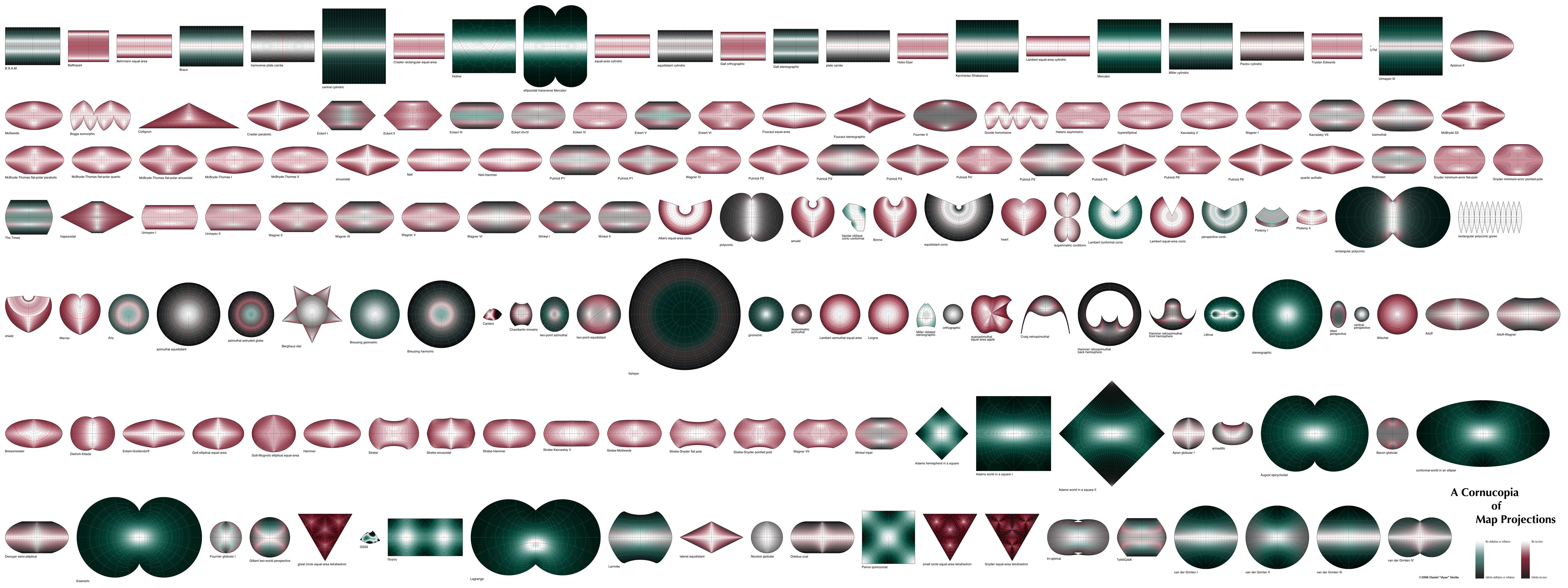
8. "A cornucopia of map projections".
9. Peters, A. B. (1978). "Uber Weltkartenverzerrunngen und Weltkartenmittelpunkte". Kartographische Nachrichten: 106–113.
10. Gott, III, J. Richard; Mugnolo, Charles; Colley, Wesley N. "Map projections for minimizing distance errors". arXiv:astro-ph/0608500v1.
11. Laskowski, P. (1997). "Distortion-spectrum fundamentals: A new tool for analyzing and visualizing map distortions". Cartographica 34 (3).
12. Airy, G.B. (1861). "Explanation of a projection by balance of errors for maps applying to a very large extent of the Earth's surface; and comparison of this projection with other projections". London, Edinburgh, and Dublin Philosophical Magazine. 4 22 (149): 409–421.

External links

• Java applet with interactive projections showing Tissot's indicatrix